In this post, we'll explore Regularization in ML with special focus on regularization in Linear Regression Algorithm, types of regularization and the underlying mathematics. Let's jump in.

Introduction to Regularization

A good machine learning model that makes accurate predictions on new unseen examples, do it by learning the underlying pattern in the training data. Across all classical ML algorithms, one thing is common — Training data got some robust underlying patterns, model parameters can be tweaked to fit that patterns in data, and those needed changes in parameter values are estimated during training via optimization algorithm.

However, as models become increasingly complex, due to increasing model parameters or ability to model the weakest patterns in data, they often begin learning not only the true patterns but also the random noise present in the training data. This phenomenon is known as overfitting and results in poor generalization.

Regularization is a family of techniques designed to prevent overfitting by controlling the complexity of a machine learning model. By applying regularization, we introduce a penalty term into the model's loss function. During loss minimization and search for global minima, this penalty discourages the model from assigning excessively large values to its parameters, forcing it to learn simpler and more robust patterns instead of memorizing the training data and overfit.

As a result, regularization enables a model to generalize better on new unseen data, enabling it to perform well.

Why Do We Exactly Need Regularization? — Past Signal, Learning Noise

To understand the need for regularization, consider what happens during model training.

Initially, each optimization step significantly reduces the model's error because the model is learning the genuine relationships present in the data. But after a certain point, however, most of the remaining error is no longer due to missing true pattern but is instead irreducible error — random noise that cannot be explained by the underlying data-generating process.

In such a situation, an unconstrained optimization algorithm which has no way of distinguishing between genuine signal and noise. With objective to minimize the loss function as much as possible. Continues to adjust model parameters, often inflating the regression coefficients to fit random fluctuations in the training data. This is precisely how overfitting occurs.

Now the model is just mugging up the training data and not aware of true pattern in data. Hence the resultant model will have high variance and poor generalization on new unseen data.

Here, regularization comes to rescue. It changes the optimization objective by introducing a penalty term into the loss function. The optimization algorithm must now reduce the prediction error while simultaneously avoiding unnecessarily large coefficients. This additional constraint:

• discourages overly complex models,
• prevents overfitting, and
• produces models that generalize much better to new unseen data.

In essence, regularization helps the optimization algorithm to find that sweet-spot of best possible generalization without overfitting the training data.

For easy understanding of regularization let's see how it applies in the most simplest machine learning algorithm.

Regularization in Linear Regression

In Linear Regression, the model learns a set of coefficients (weights) that defines the relationship between the input features and the target variable. During training, the optimization algorithm attempts to minimize the loss function — typically the Residual Sum of Squares (RSS) or Mean Squared Error (MSE).

During training, if the model is allowed to minimize the training error without any constraints, it often assigns very large values to the regression coefficients in an attempt to fit every minor fluctuation in the training data, including random noise. When model starts to fit noise in data, it inflates the coefficients and those inflated values don't represent true contribution of that feature in the model's prediction. Results in a garbage model. High variance model with poor generalization.

Regularization addresses this issue by modifying the loss function to penalize large coefficient values. Instead of focusing solely on minimizing prediction error, the optimization algorithm must now balance two competing objectives:

• Minimize the prediction error.
• Keep the model coefficients reasonably small.

By constraining the coefficients, the model learns the dominant trends in the data while ignoring the insignificant noise, leading to better generalization on unseen data. We'll soon prove this by an example.

For Linear Regression, three widely used regularization techniques are:

1. Ridge Regression (L2 Regularization)
2. Lasso Regression (L1 Regularization)
3. Elastic Net Regression (L1 + L2 Regularization)

Let's jump in and uncover Ridge Regularization.

Ridge Regression (L2 Regularization)

Ridge Regression, also known as L2 Regularization, is one of the most widely used regularization techniques for linear regression.

The penalty term introduced by ridge regression into the loss function increases as the magnitude of the model coefficients increases, preventing the optimization algorithm from assigning unnecessarily large weights to the features.

As a result, Ridge Regression trains a simpler and more stable model that captures the underlying trend in the data rather than memorizing random noise.

One of the key characteristics of Ridge Regression is that it introduces a small amount of bias into the model in exchange for a significant reduction in variance. Although the training error may increase slightly, the resulting model is typically much more robust and produces better predictions on new data. This is a classic example of the Bias–Variance Trade-off, where accepting a small increase in bias leads to a substantial improvement in generalization due to significant drop in variance.

Mathematical Formulation

Mathematically, Ridge Regression modifies the standard Least Squares objective function by adding a penalty proportional to the sum of the squared values of the coefficients. This penalty forces the optimization algorithm to keep the coefficients small unless a large coefficient is strongly supported by the data.

The Ridge regression loss function is given by:

$\hspace{3.5cm} L(w) = \underbrace{\sum_{i=1}^{n}(y_i-X_i.w)^2}_{\text{Prediction Error}} + \lambda.\underbrace{\sum_{j=1}^{p}w_j^{2}}_{\text{L2 Penalty}}$

where:

• The first term is the MSE loss.
• The second term shrinks the coefficients by penalizing large values.
• $λ$ is a hyperparameter that controls the extent of regularization. Its value ranges from $0$ to $∞$.
  • Higher $λ$ → More shrinkage.
  • Very High $λ$ may cause Underfitting.
  • $λ = 0$ → No Regularization; Same as usual Linear Regression.
  • Optimal $λ$ is found using Cross-Validation.

NOTE: Ridge Regression shrinks the coefficients toward zero but never exactly to zero. Every feature remains in the model, although features with little predictive power receive very small coefficients.

This property makes Ridge Regression particularly effective when dealing with:

• Multicollinearity (highly correlated features)
• High-dimensional datasets with many features
• Models that exhibit high variance and overfitting

In the following sections, we'll see Ridge Regularization in action, derive the closed-form solutions for n-dimensional data and how does $\lambda$ controls the magnitude of regularization.

Some easy mathematics on its way, Sit tight!

An Example of Ridge Regression

Let's see by an example how ridge rgularization helps achieve generalisation even on small datasets. Let’s start by generating a synthetic non-linear 2-D data of 1000 datapoints and draw a sample of 80 datapoints from it.

Now let's fit a Polynomial Regression (of degree 15) on this data and note the R2 Score on training and testing data and the coefficients values. Then fit a Ridge Regression $(λ = 20)$ on that same data and compare similar metrices.

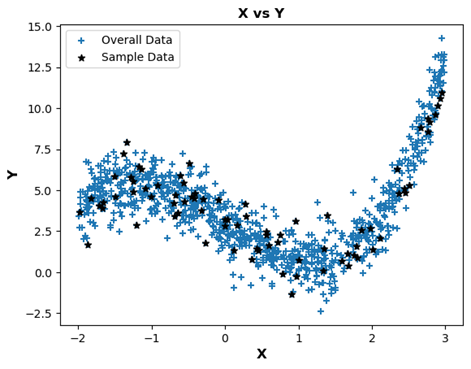
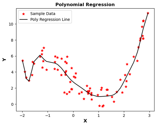
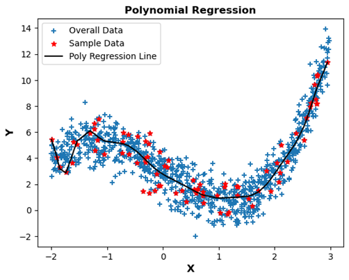
We can clearly see that the Polynomial Regression is overfitting the Training data and not generalizing well on new unseen data. Now let’s fit the Ridge Regression.

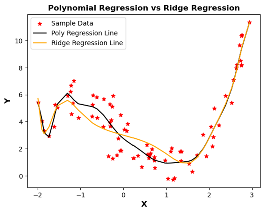
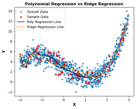
Now, we can clearly see that Ridge Regression Line is generalizing better than the Polynomial Regression Line. Now let’s compare them!

Check the difference between coefficients of Polynomial Regression and Ridge Regression. Ridge Regression has reduced coefficients values (how? – we’ll soon uncover out the mathematics).

Ridge Regression has reduced the effect of all the coefficients on the model’s outcome, hence preventing the model from fitting the noise in the data and hence preventing overfitting.

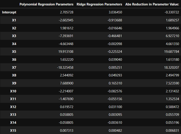
Now, let’s compare Training and Test R2 Scores for both the models.

We can clearly see, in case of Polynomial Regression the difference between training and test R2 Score is a huge $5$. Whereas, in case of Ridge Regression, this difference is significantly reduced (only $0.4$), although the R2 Score for training is also slightly reduced compared to the other model. But this is what we do by applying regularization - introduce a small bias to significantly reduce variance, hence preventing overfitting and achieving generalization.

Derivation of Closed Form Solution of Ridge Regression - For 2D Data

Let’s say we have $X$ as a single input feature and $Y$ as target variable, we want to fit a Ridge Regression over this data. Now the closed form solution can be given as:

$\hspace{3.5cm} \hat{Y} = mX + b$

where:

$\hspace{2cm} \boxed{ \quad b = \bar{Y} - m\bar{X}; \quad m = \frac{\sum_{i=1}^{n} (Y_i - \bar{Y})(X_i - \bar{X})}{\sum_{i=1}^{n} (X_i - \bar{X})^2 + \lambda} \quad}$

where:

• $\bar{X}$ : mean of input variable X
• $\bar{Y}$ : mean of target variable Y

The Loss Function for Ridge Regression can be given as:

$\hspace{3.5cm} L(m,b) = \text{MSE} + \text{Penalty Term }(\lambda)$

$\hspace{3.5cm} L(m,b) = \frac{1}{n} \sum_{i=1}^{n} (Y_i - \hat{Y}_i)^2 + \lambda \times m^2$

$\hspace{3.5cm} L(m,b) = \frac{1}{n} \sum_{i=1}^{n} (Y_i - mX_i - b)^2 + \lambda \times m^2$

Now differentiating $L(m, b)$ with respect to $b$ and equating it to zero:

$\hspace{3.5cm} \frac{\partial L(m,b)}{\partial b} = -\frac{2}{n} \sum_{i=1}^{n} (Y_i - mX_i - b)$

$\hspace{3.5cm} \frac{\partial L(m,b)}{\partial b} = -2(\bar{Y} - m\bar{X}) + \frac{2}{n} \sum_{i=1}^{n} b$

$\hspace{3.5cm} \frac{\partial L(m,b)}{\partial b} = -2(\bar{Y} - m\bar{X}) + \frac{2}{n} \cdot nb$

$\hspace{3.5cm} \frac{\partial L(m,b)}{\partial b} = -2(\bar{Y} - m\bar{X} - b)$

$\hspace{3.5cm} \frac{\partial L(m,b)}{\partial b} = -2(\bar{Y} - m\bar{X} - b) = 0$

$\hspace{3.5cm} \boxed{b = \bar{Y} - m\bar{X}}$

Now differentiating $L(m, b)$ with respect to $m$ and equating it to zero:

$\hspace{0.5cm} \frac{\partial L(m,b)}{\partial m} = \frac{2}{n}\sum_{i=1}^{n} \left(Y_i - mX_i - \bar{Y} + m\bar{X}\right) \cdot \left(-X_i + \bar{X}\right) + 2\lambda m$

$\hspace{0.5cm} \frac{\partial L(m,b)}{\partial m} = \frac{-2}{n}\sum_{i=1}^{n} \left(Y_i - \bar{Y} - m(X_i - \bar{X})\right) \cdot (X_i - \bar{X}) + 2\lambda m$

$\hspace{0.5cm} \frac{\partial L(m,b)}{\partial m} = \frac{-2}{n}\sum_{i=1}^{n} \left[ (Y_i - \bar{Y}) \cdot (X_i - \bar{X}) - m(X_i - \bar{X})^2 \right] + 2\lambda m$

$\hspace{0.5cm} \frac{\partial L(m,b)}{\partial m} = \frac{-2}{n}\sum_{i=1}^{n} (Y_i - \bar{Y}) \cdot (X_i - \bar{X}) - \frac{-2m}{n}\sum_{i=1}^{n} (X_i - \bar{X})^2 + 2\lambda m$

$\hspace{0.5cm} \frac{\partial L(m,b)}{\partial m} = \frac{-2}{n}\sum_{i=1}^{n} (Y_i - \bar{Y}) \cdot (X_i - \bar{X}) - \frac{-2m}{n}\sum_{i=1}^{n} (X_i - \bar{X})^2 + 2\lambda m = 0$

$\hspace{3.5cm} \boxed{m = \frac{\frac{1}{n}\sum_{i=1}^{n} (Y_i - \bar{Y}) \cdot (X_i - \bar{X})}{\frac{1}{n}\sum_{i=1}^{n} (X_i - \bar{X})^2 + \lambda}}$

Here, $λ$ is model hyperparameter. We can find the optimum value for $λ$ using Cross-Validation. Through the above formula we can see that:

More the value of $λ$, more the Regularization and more the decrease in value of $m$

How Gradient Descent Applies in Ridge Regression - Derivation for n-D Data

Let’s say we have input feature space $X$ as ${X_{1},X_{2},X_{3},\ldots.,X_{m}}$ and $Y$ as the target variable. Say, training data includes $n$ records. We want to fit a Ridge Regression over this data using Gradient Descent as an optimization algorithm. Given the loss function be:

$\hspace{3.5cm} L(\mathbf{w}) = \frac{1}{2n}\sum_{i=1}^{n}\left(Y_i - \hat{Y}_i\right)^2 + \frac{\lambda}{2}\sum_{j=1}^{m} w_j^2$

$\hspace{3.5cm} L(\mathbf{w}) = \frac{1}{2n}\sum_{i=1}^{n}\left(Y_i - \mathbf{X}_i\mathbf{w}\right)^2 + \frac{\lambda}{2}\sum_{j=1}^{m} w_j^2$

Where:

• $\mathbf{w} = [w_0, w_1, w_2, \ldots, w_m]^T$

The Solution in the form of Weight Update Rules can be given as:

$\hspace{3.5cm} \boxed{w_0(\text{new}) = w_0(\text{old}) - \eta \times \frac{1}{n}\sum_{i=1}^{n}\left(\mathbf{X}_i\mathbf{w} - Y_i\right)}$

And, for $w_1, w_2, w_3, \ldots, w_m$:

$\hspace{3.5cm} \boxed{w_j(\text{new}) = w_j(\text{old}) - \eta \times \left[ \frac{1}{n}\sum_{i=1}^{n}\left(\mathbf{X}_i\mathbf{w} - Y_i\right)X_{ij} + \lambda w_j \right]}$

where:

• $\eta$ = Learning rate
• $j = 1, 2, 3, 4, \ldots, m$
• $X_{ij}$ = $j^{\text{th}}$ input feature of $i^{\text{th}}$ training record

Derivation:

The Loss Function for Ridge Regression can be given as:

$\hspace{3.5cm} L(\mathbf{w}) = \text{MSE} + \text{Penalty Term} (\lambda)$

$\hspace{3.5cm} L(\mathbf{w}) = \frac{1}{2n}\sum_{i=1}^{n}\left(Y_i - \hat{Y}_i\right)^2 + \frac{\lambda}{2}\sum_{j=1}^{m} w_j^2$

$\hspace{3.5cm} \boxed{\quad L(\mathbf{w}) = \frac{1}{2n}\sum_{i=1}^{n}\left(Y_i - \mathbf{X}_i\mathbf{w}\right)^2 + \frac{\lambda}{2}\sum_{j=1}^{m} w_j^2 \quad}$

where:

• $m$ = total number of input features
• $n$ = total of number of records in training set

NOTE: Intercept $w_{0}$ is excluded from the Penalty Term

To apply Gradient descent, we need to iteratively update the intercept and coefficients. The update rule for Intercept $w_{0}$ be:

$\hspace{3.5cm} w_0(\text{new}) = w_0(\text{old}) - \eta \times \frac{\partial L}{\partial w_0}$

Finding the derivative of $L$ w.r.t $w_{0}$ or $w_{intercept}$:

$\hspace{3.5cm} \frac{\partial L}{\partial w_0} = \frac{\partial}{\partial w_0} \left( \frac{1}{2n}\sum_{i=1}^{n}\left(Y_i - \mathbf{X}_i\mathbf{w}\right)^2 + \frac{\lambda}{2}\sum_{j=1}^{p}w_j^2 \right)$

$\hspace{3.5cm} \frac{\partial L}{\partial w_0} = -\frac{2}{2n}\sum_{i=1}^{n}\left(Y_i - \mathbf{X}_i\mathbf{w}\right) + 0$

$\hspace{3.5cm} \frac{\partial L}{\partial w_0} = \frac{1}{n}\sum_{i=1}^{n}\left(\mathbf{X}_i\mathbf{w} - Y_i\right)$

Hence, the Update Rule for Intercept is:

$\hspace{3.5cm} \boxed{\quad w_0(\text{new}) = w_0(\text{old}) - \eta \times \frac{1}{n}\sum_{i=1}^{n}\left(\mathbf{X}_i\mathbf{w} - Y_i\right) \quad}$

Now, the update rule for Coefficient $w_{j}$ (where $j$ from $1$ to $m$) be:

$\hspace{3.5cm} w_j(\text{new}) = w_j(\text{old}) - \eta \times \frac{\partial L}{\partial w_j}$

Finding the derivative of $L$ w.r.t $w_{j}$ or $w_{\text{coefficient of } X_j}$:

$\hspace{3.5cm} \frac{\partial L}{\partial w_j} = \frac{\partial}{\partial w_j} \left( \frac{1}{2n}\sum_{i=1}^{n}\left(Y_i - \mathbf{X}_i\mathbf{w}\right)^2 + \frac{\lambda}{2}\sum_{j=1}^{m}w_j^2 \right)$

$\hspace{3.5cm} \frac{\partial L}{\partial w_j} = -\frac{2}{2n}\sum_{i=1}^{n}\left(Y_i - \mathbf{X}_i\mathbf{w}\right)X_{ij} + \frac{2\lambda}{2}w_j$

$\hspace{3.5cm} \frac{\partial L}{\partial w_j} = \frac{1}{n}\sum_{i=1}^{n}\left(\mathbf{X}_i\mathbf{w} - Y_i\right)X_{ij} + \lambda w_j$

Hence, the Update Rule for Coefficients $w_1, w_2, w_3, \ldots, w_m$ is:

$\hspace{3.5cm} \boxed{ \quad w_j(\text{new}) = w_j(\text{old}) - \eta \times \left[ \frac{1}{n}\sum_{i=1}^{n}\left(\mathbf{X}_i\mathbf{w} - Y_i\right)X_{ij} + \lambda w_j \right] \quad}$

where:

• $\eta$ = Learning rate
• $j = 1, 2, 3, 4, \ldots, m$
• $X_{ij}$ = $j^{\text{th}}$ feature of $i^{\text{th}}$ training record

For all $m$ coefficients together, the Update rule in matrix format can be given as:

$\hspace{3.5cm} \boxed{\quad \mathbf{w}(\text{new}) = \mathbf{w}(\text{old}) - \eta \times \left[ \frac{1}{n}\mathbf{X}^T(\mathbf{X}\mathbf{w} - \mathbf{Y}) + \lambda \mathbf{w} \right] \quad }$

See how $- \lambda w_{j}$ term coming from the derivative of Penalty Term, adds to further reduction in value of model weights ($w_{j}$) on each update. Now the aim on every weight update is not just reduction in prediction error but to also keep the model weights small. This is how Ridge Regression balances two objectives of reducing prediction error and preventing exploding model weights. Hence, preventing overfitting and attaining generalisation.

One thing must have cross your mind that, why intercept weight is not included in the Penalty Term? Let's see that next.

Why Does the Intercept ($w_{0}$) Not Included in Penalty Term?

Regularizing the intercept can shift the entire regression line, affecting the model's ability to fit the data. We want the model to be flexible enough to comfortably capture the underlying relationship between the variables. Hence regularization should solely focus on the coefficients of input variables to prevent overfitting.

Including intercept in the penalty term would force it to be smaller than it should be, merely for the sake of minimizing the cost — even if the true data naturally has a non-zero average. THIS CREATES SYSTEMATIC UNDERFITTING. It can:

• Shift the entire model towards the origin.
• Distort the learned relationship between input features and the target.
• Hurt model performance, especially if data is not centred around zero.

In next post, we'll cover the most famous "Lasso Regularization".