In this second post, we'll explore Lasso Regularization in detail. How it works? Optimization technique used for solution finding? Why it shrinks coefficients to zero and induce sparsity? Geometric Interpretations of Lasso Regularization. Sound's interesting? Let's jump in.

Lasso Regression - L1 Regularization

LASSO stands for “Least Absolute Shrinkage and Selection Operator”. It is a type of regularization technique used in linear regression and other models to prevent overfitting and perform feature selection. In Lasso Regression, the cost function of linear Regression is modified by adding a Penalty Term. This penalty term is nothing but sum of absolute values of the model coefficients.

Lasso Loss Function:

$\hspace{3.5cm} \boxed{ \quad L(w) = \underbrace{\sum_{i=1}^{n}(y_i-X_i.w)^2}_{\text{Prediction Error}} + \lambda.\underbrace{\sum_{j=1}^{p}|w_j|}_{\text{L1 Penalty}} \quad}$

where:

• $\sum(y_i-X_i.w)^2$ → Mean Squared Error (MSE)
• $\lambda.\sum|w_j|$ → L1 Penalty (sum of absolute values)
• $\lambda$ → Strength of regularization

NOTE: The intercept $w_0$ is not included in the Penalty Term.

Key Features

Why Use Lasso Variant over Vanilla Linear Regression?

1. Prevents Overfitting: prevents model to fit random noise in data and cause exploding coefficients.
2. Automatic Feature Selection: features with smaller coefficients are already contributing less in predictions, they are less important. Lasso makes their coefficients exactly zero. Hence they are removed from the model.
3. Slash Model Complexity: Useful when data have many input features but only a few are useful.

Mathematical Formulation & Solution Using Coordinate Descent

Lasso Regression modifies the standard linear regression objective by adding a ‘Penalty Term’ which is sum of the absolute values of the coefficients. We know, Lasso Loss Function:

$\hspace{3.5cm} L(w) = \frac{1}{2n}\underbrace{\sum_{i=1}^{n}(y_i-X_i.w)^2}_{\text{Prediction Error}} + \lambda.\underbrace{\sum_{j=1}^{p}|w_j|}_{\text{L1 Penalty}}$

Given:

• $X \in R^{m \times p}$ is the input matrix. Total $p$ input features.
• $n$ is the number of records in training set.
• $y \in R^{m}$ is the target vector.
• $w \in R^{p}$ is the vector of coefficients (excluding intercept).
• $λ ≥ 0$ is hyperparameter; controlling the amount of shrinkage.

One big issue in finding solution for the above cost function – LOSS FUNCTION IS NOT DIFFERENTIABLE AT 0. Hence Gradient Descent Optimization Algorithm can't work.

Gradient Descent (GD) requires a single, definitive slope at every point to update the weights. Lasso Regression prevents this because of the L1 penalty term breaks the mathematical rule of differentiation. Mathematical rule that, for a function to have a derivative at a point, the slope approaching from the left must equal the slope approaching from the right. The derivative at $w_j = 0$ is undefined.

When Gradient Descent runs its weights update step. If a weight hits exactly $0.0$, the algorithm requests the value of $\frac{\partial \text{Loss}}{\partial w}$. The computer receives an undefined mathematical error (NaN or division failure), causing standard Gradient Descent to break down.

So, the objective is convex but not differentiable. Due to this reason, we don’t have a Closed-Form Solution in Lasso Regression. Here we’ll utilise a new optimization technique – “Coordinate Descent”. Let's quickly see what it is.

Coordinate Descent Algorithm

Coordinate Descent is an Optimization Algorithm that minimizes a multivariate objective function by iteratively optimizing it along one coordinate (variable) at a time while keeping all other coordinates fixed. It is particularly useful for high-dimensional problems where gradient-based methods may be computationally expensive.

Coordinate Descent (CD) updates only one variable per iteration, unlike GD which updates all the variables in an iteration. It can also work with non-differentiable functions (depending on variant). Highly efficient for large-scale problems. Convergence guaranteed under certain conditions like convexity and smoothness.

NOTE: In Lasso Regression implementation of Scikit-learn, Coordinate Descent Algorithm is used.

Types of Coordinate Descent:

1. Cyclic Coordinate Descent: Updates variables in a fixed order (e.g., w1, w2, …, wp).
2. Randomized Coordinate Descent: Picks a variable randomly in each iteration.
3. Greedy Coordinate Descent: Search and selects the variable that leads to the largest descent.

Let's apply Coordinate Descent in Lasso Regression to find the optimal solution.

Lasso Regression Solution - via CD

The coefficient update step for coefficient $w_j$ in an iteration of Coordinate Descent can be given as:

$\hspace{3.5cm} \boxed{ \quad w_j^{k + 1} = \underset{y \in \mathbb{R}}{\operatorname{arg\,min}} \; L\left(w_0^k, w_1^k, \dots, w_{j - 1}^k, y, w_{j + 1}^k, \dots, w_p^k\right) \quad }$

where:

• $k + 1$ – Current Iteration; $k$ – Previous Iteration
• $w_0^k, w_1^k, w_2^k, w_3^k, \dots,$ = values of coefficients after $k$ iterations
• Except for $w_j$ all other coefficients are fixed in the above equation
• $w_j^{k+1}$ = updated value of coefficient $w_j$, after $k + 1^{th}$ iterations

After this $k + 1^{th}$ iterations, updated coefficients are:

$\hspace{3.5cm} \boxed{ \quad W^{k + 1} = (w_0^k, w_1^k, \dots, w_{j - 1}^k, w_{j}^{k+1}, w_{j + 1}^k, \dots, w_p^k) \quad }$

Because, $w_j$ was the only coefficients which was updated in $k + 1^{th}$ iteration.

Exact Update Step can be given as:

In an optimization iteration, for coefficient $w_j$, Lasso update is:

$\hspace{3.5cm} \boxed{ \quad w_j(\text{new}) = \text{Soft Thresholding} \left( \frac{1}{n} \sum_{i = 1}^{n} \left( y_i - \mathbf{X}_{-j} \mathbf{w}_{-j} \right) X_{ij}, \, \lambda \right) \quad}$

where:

• $ŷ_{−j}$ is the model's prediction without the contribution of $w_j$.
• Soft Thresholding means:

$\hspace{3.5cm} \boxed{ \quad S(z, \lambda) = \begin{cases} z - \lambda & \text{if } z > \lambda \\ z + \lambda & \text{if } z < -\lambda \\ 0 & \text{if } |z| \leq \lambda \end{cases} \quad}$

How do we arrive at this weird looking Soft Thresholding Operation? And how this operation works? Let's see this next and derive these results.

Derivation

The Loss Function for Lasso Regression is:

$\hspace{3.5cm} L(w) = \frac{1}{2n}\underbrace{\sum_{i=1}^{n}(y_i-X_i.w)^2}_{\text{Prediction Error}} + \lambda.\underbrace{\sum_{j=1}^{p}|w_j|}_{\text{L1 Penalty}}$

$\hspace{3.5cm} L(\mathbf{w}) = \frac{1}{2n} \sum_{i = 1}^{n} \left( y_i - \left( w_0 + \sum_{j = 1}^{p} X_{ij} w_j \right) \right)^2 + \lambda \sum_{j = 1}^{p} |w_j|$

$\hspace{1.5cm} L(\mathbf{w}) = \frac{1}{2n} \sum_{i = 1}^{n} \left( y_i - \left( w_0 + X_{i1} w_1 + X_{i2} w_2 + X_{i3} w_3 + \dots + X_{ip} w_p \right) \right)^2 + \lambda \sum_{j = 1}^{p} |w_j|$

Now, differentiate $L(w)$ w.r.t $w_j$ keeping other coefficients fixed. Then, find the value of $w_j$ for which the derivative is zero.

$\hspace{0cm} \frac{\partial L(\mathbf{w})}{\partial w_j} = \frac{\partial}{\partial w_j} \left( \frac{1}{2n} \sum_{i = 1}^{n} \left( y_i - \left( w_0 + X_{i1} w_1 + X_{i2} w_2 + \dots + X_{ip} w_p \right) \right)^2 + \lambda \sum_{k = 1}^{p} |w_k| \right)$

$\hspace{0cm} \frac{\partial L(\mathbf{w})}{\partial w_j} = \frac{-2}{2n} \sum_{i = 1}^{n} \left( y_i - \left( w_0 + X_{i1} w_1 + \dots + X_{ij} w_j + \dots + X_{ip} w_p \right) \right) X_{ij} + \lambda \operatorname{sign}(w_j)$

$\hspace{0cm} \frac{\partial L(\mathbf{w})}{\partial w_j} = \frac{-1}{n} \sum_{i = 1}^{n} \left( y_i - \left( w_0 + X_{i1} w_1 + \dots + X_{ij} w_j + \dots + X_{ip} w_p \right) \right) X_{ij} + \lambda \operatorname{sign}(w_j)$

Equating above equation with $0$ to get the value of $w_j$ for which it is minimum:

$\hspace{0.5cm} \frac{\partial L(\mathbf{w})}{\partial w_j} = \frac{-1}{n} \sum_{i = 1}^{n} \left( y_i - \left( w_0 + X_{i1} w_1 + \dots + X_{ij} w_j + \dots + X_{ip} w_p \right) \right) X_{ij} + \lambda \operatorname{sign}(w_j) = 0$

$\hspace{0.5cm} \frac{-1}{n} \sum_{i = 1}^{n} \left( y_i - \left( w_0 + X_{i1} w_1 + \dots + X_{i.j-1} w_{j-1} + X_{i.j+1} w_{j+1} + \dots + X_{ip} w_p \right) \right) X_{ij} + \left( \frac{1}{n} \sum_{i = 1}^{n} (X_{ij} w_j) . X_{ij} \right) + \lambda \operatorname{sign}(w_j) = 0$

$\hspace{0.5cm} \frac{-1}{n} \sum_{i = 1}^{n} \left( y_i - \sum_{j^{th} \text{feature excluded}} X_{i-j} w_{-j} \right) X_{ij} + \left( \frac{1}{n} \sum_{i = 1}^{n} X_{ij}^2 \right) w_j + \lambda \operatorname{sign}(w_j) = 0$

Taking out the $w_j$ term from the summation, where $y_i - \sum X_{i.-j} w_{-j}$ calculating residuals, excluding the effect of $j^{th}$ input feature and $w_j$ coefficient on the prediction:

$\hspace{0.5cm} \left( \frac{1}{n} \sum_{i = 1}^{n} X_{ij}^2 \right) w_j = \frac{1}{n} \sum_{i = 1}^{n} \left( y_i - X_{i-j} w_{-j} \right) X_{ij} - \lambda \operatorname{sign}(w_j) = 0$

$\hspace{0.5cm} w_j . \frac{1}{n} \sum_{i = 1}^{n} X_{ij}^2 = \frac{1}{n} \sum_{i = 1}^{n} \left( y_i - X_{i-j} w_{-j} \right) X_{ij} - \lambda \operatorname{sign}(w_j)$

Now, Assuming input feature $X_j$ is standardized. Hence $\sum_{i = 1}^{n} X_{ij}^2 = 1$ So, the final update step for $w_j$ is:

$\hspace{3.5cm} \boxed{w_j = \frac{1}{n} \sum_{i = 1}^{n} \left( y_i - X_{i-j} w_{-j} \right) X_{ij} - \lambda \operatorname{sign}(w_j)}$

NOTE: Sign of $w_j$ is the same as the sign of $\frac{1}{n} \sum_{i = 1}^{n} \left( y_i - X_{i-j} w_{-j} \right) X_{ij}$ (when $w_j ≠ 0$). How? We'll discuss this.

The above equation is equivalent to “Soft Thresholding Operation”. So,

$\hspace{3.5cm} \boxed{ \quad w_j = \text{Soft Thresholding} \left( \frac{1}{n} \sum_{i = 1}^{n} \left( y_i - \mathbf{X}_{i-j} \mathbf{w}_{i-j} \right) X_{ij}, \, \lambda \right) \quad}$

Let's take a quick detour to understand "Soft Thresholding" - the operation that appears naturally in Lasso Regression due to L1-penalty and shrinks coefficients (some to zero) and induce sparsity.

Soft Thresholding Operation

Soft Thresholding (also called shrinkage) is a mathematical operation used in signal processing and optimization, particularly in sparse regressions. It shrinks values towards zero, hence effectively inducing sparsity.

Think of it like a special function, given a scalar $y$ and a threshold $λ > 0$, the soft-thresholding operator $S_λ (y)$ is defined as:

$\hspace{3.5cm} \boxed{ \quad S_λ (y) = \operatorname{sign}(y) . \text{max}(|y| - \lambda, 0) \quad }$

Interpretation:

• If $|y| > \lambda \rarr S_λ (y) = \operatorname{sign}(y) . (y-\lambda)$ means $y$ is shrunk towards zero.
• If $|y| \leq \lambda \rarr S_λ (y) = 0$ means $y$ is thresholded to zero.

Soft Thresholding Operation appears naturally in Coordinate Descent based optimization for lasso regression, and its all because of L1-penalty term.

If we look closely, in Lasso Regression, our sole job is to minimize the loss function and find the optimal set of coefficients. Its L1-penalty term in loss function that leads to application of soft thresholding operation on ordinary least-squares regression solution (a solution without any regularization) of the problem. This can be denoted as:

$\hspace{3.5cm} \boxed{ \quad \beta_j \rarr S_\lambda(\beta_j^{\text{OLS}}) \quad }$

Here, $\beta_j^{\text{OLS}}$ is the roughly equal to ordinary least-squares solution without regularization (roughly because we are still missing the contribution of $X_j$ in residual calculation).

So, you see the hidden master that shrinks coefficients and causes sparsity? Yes, its Soft Thresholding Operation that comes naturally due to L1-penalty term in Coordinate Descent based optimization, because the loss function is not differentiable at 0 and we cannot use Gradient Descent based optimization.

Back to Derivation

One question still remains. How did we go from below equation to Soft Thresholding Operation? Let’s see.

$\hspace{3.5cm} w_j = \frac{1}{n} \sum_{i = 1}^{n} \left( y_i - X_{i-j} w_{-j} \right) X_{ij} - \lambda \operatorname{sign}(w_j)$

$\hspace{3.5cm} \boxed{ \quad w_j = z - \lambda \operatorname{sign}(w_j) \quad }$

We know that, when we apply Coordinate Descent, we make single weight update in an iteration keeping all other coefficients fixed. To solve the above equation we know the $\operatorname{sign}(w_j)$.

Now here the problem arise. Coefficient $w_j$ is a variable and $\operatorname{sign}(w_j)$ is the sign of optimised or updated $w_j$, but we don’t know what would be the future sign of $w_j$, will it be $+ve$ or $-ve$ or no sign i.e., $0$.

What if I tell you that their is a hack to find it via "$z$" i.e., $\frac{1}{n} \sum_{i = 1}^{n} \left( y_i - X_{i-j} w_{-j} \right) X_{ij}$.

Let's see for different possible values of $\operatorname{sign}(w_j)$ how does the optimal solution looks:

I. If updated $w_j > 0$ i.e., $\operatorname{sign}(w_j)$ be $+ve$:

• Sub-gradient $∂∣w_j∣ = +1$
• Optimality condition:

$\hspace{3.5cm} w_j = \frac{1}{n} \sum_{i = 1}^{n} \left( y_i - X_{i-j} w_{-j} \right) X_{ij} - \lambda$

$\hspace{3.5cm} \boxed{ \quad w_j = z - \lambda \quad }$

Requirements:

• For updated $w_j \text{ to be +ve } \rarr z > λ$, otherwise $w_j \leq 0$ and would contradict the assumption of $w_j > 0$.
• Means updated $w_j > 0$, only and only when, $z > λ$. Since $λ \geq 0$, $z$ must be positive for $w_j > 0$.
• This way $\operatorname{sign}(w_j)$ aligns with $\operatorname{sign}(z)$.

II. If updated $w_j < 0$ i.e., $\operatorname{sign}(w_j)$ be $-ve$:

• Sub-gradient $∂∣w_j∣ = -1$
• Optimality condition:

$\hspace{3.5cm} w_j = \frac{1}{n} \sum_{i = 1}^{n} \left( y_i - X_{i-j} w_{-j} \right) X_{ij} + \lambda$

$\hspace{3.5cm} \boxed{ \quad w_j = z + \lambda \quad }$

Requirements:

• For updated $w_j \text{ to be -ve } \rarr z < -λ$, otherwise $w_j \geq 0$ and would contradict the assumption of $w_j < 0$.
• Means updated $w_j < 0$, only and only when, $z < -λ$. Since $λ \geq 0$, $z$ must be negative for $w_j < 0$.
• This way $\operatorname{sign}(w_j)$ aligns with $\operatorname{sign}(z)$.

III. If updated $w_j = 0$:

• Sub-gradient $∂∣w_j∣ \in [-1, 1]$
• Optimality condition:

$\hspace{3.5cm} \left| \frac{1}{n} \sum_{i = 1}^{n} \left( y_i - X_{i-j} w_{-j} \right) X_{ij} \right| \leq \lambda$

$\hspace{3.5cm} \boxed{ \quad |z| \leq \lambda \quad }$

Requirements:

• For updated $w_j \text{ to be 0 } \rarr |z| \leq \lambda$, otherwise $w_j \neq 0$ and would contradict the assumption of $w_j = 0$.

Hence the equation from derivation can be re-written as:

$\hspace{3.5cm} \boxed{ \quad w_j = \begin{cases} z - \lambda & \text{if } z > \lambda \\ z + \lambda & \text{if } z < -\lambda \\ 0 & \text{if } |z| \leq \lambda \end{cases} \quad}$

Look closely this is nothing but Soft Thresholding Operation on $z$ and $\lambda$. Hence:

$\hspace{3.5cm} \boxed{ \quad w_j = \text{Soft Thresholding} \left( \frac{1}{n} \sum_{i = 1}^{n} \left( y_i - \mathbf{X}_{i-j} \mathbf{w}_{i-j} \right) X_{ij}, \, \lambda \right) \quad}$

So, we just completed a very crucial derivation and also uncovered what actually causes shrinkage of coefficients.

For extra curious beings, I have written an separate article, where I have geometrically explained how $\operatorname{sign}(w_j)$ aligns with $\operatorname{sign}(z)$. Do check out!

Geometric Intuition of how sign(𝑤ⱼ) aligns with sign(z) in Lasso Regression

What Causes Shrinking of Weights In Lasso?

Although via derivation this question can be answered best. I you request for a quick read for in-depth understanding. In this section let's summarise our understanding.

The main reason behind Lasso Regression causing shrinkage of coefficients and reducing some coefficients to absolute zero is "Soft Thresholding Operation" that appears naturally in its solution, due to L1-penalty term in the Lasso Cost Function, for which optimal solution is found via Coordinate Descent based optimization.

Soft Thresholding Operation causes shrinkage and results in the coefficients being reduced—by a factor of $λ$ towards zero, promoting sparsity in the model.

Effect of Soft Thresholding Operation be:

• Large weights $(∣z∣ > λ)$ are pulled toward zero by $λ$.
• Small weights $(∣z∣ ≤ λ)$ are made absolute zero.

NOTE: Small coefficient of a input feature means the feature has low predictive power and small effect on the target variable. We can get rid of them.

Intuition: The L1 penalty "steals" $λ$ units of magnitude from each weight. If the weight is too small i.e., $|w_j| \leq \lambda$, it is set to $0$. Weak features are eliminated. Strong features are retained but penalized.

This also explains how Lasso helps in "Feature Selection".

Geometric Interpretation

To geometrically interpret the Lasso Regression, we need to view it as a constrained optimization problem. In Lasso, we aim to minimize: Least-squares loss + L1 Penalty

The least-squares loss forms a convex, smooth quadratic bowl in the parameter space. Whereas, the L1-penalty corresponds to a diamond-shaped constraint region (non-smooth at the axes due to the absolute value function i.e., $|x|$). Hence, we need to optimize the least-squares loss while satisfying the constraint imposed by the L1 penalty.

Geometrically, this means finding the point on the L1 constraint boundary where the quadratic loss is minimum.

Check the below graph. Showing contours of leas-square loss and penalty constraint boundaries of Ridge and Lasso Regression in a 2-D plot:

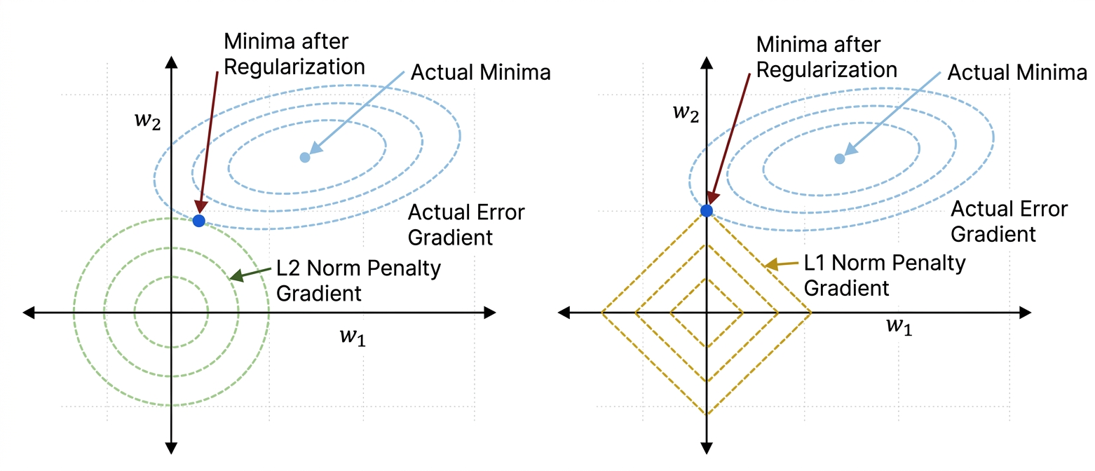
Geometric Interpretations of i. Ridge (left) and ii. Lasso Regression (right)

The least-square loss part of the objective function makes elliptical contours in weight space. Example for a lasso regression with 2 feature coefficients to optimize, a 2-D ellipse centred at the least-squares solution. Coefficient values at the centre of these elliptical contours cause overfitting. Each point on the contour yields same residual error.

The L1-penalty constraint region (when viewed as a constrained optimization problem) forms a diamond (or rhombus) in 2-D weight space.

Geometrically, the point of optimal solution is the point where the elliptical contours of least-square loss just touch the diamond-shaped constraint region of L1-penalty.

For Lasso Regression, these point of contacts are often at the corner of that diamond and not sides. These corners represent points where one or more coefficients are exactly zero. This is why Lasso promotes sparsity.

It is geometrically more likely that the minima occurs at or near the corners.

Contrast with Ridge Regression

Ridge Regression uses an L2-penalty constraint, which forms a circular constraint (or spherical boundary in higher dimensions).

The intersection of circles with ellipses is less likely to hit axes. So in ridge regression, coefficients typically shrink but do not set them to zero.

Here, we are done with Lasso Regression. Next we'll jump into "Elastic-Net Regression" - which offers the best of both worlds.