In this post, we'll see the geometric intuition of how $\text{sign}(w_j)$ aligns with $\text{sign}(z)$ in Lasso Regression. This is an important detail that arise while deriving the optimal solution for Lasso Regression via Coordinate Descent based optimization. Their comes a defining point where solution turns to Soft Thresholding Operation for calculating optimal $w_j$, because $\text{sign}(w_j)$ aligns with $\text{sign}(z)$.

For better understanding take a quick look at Lasso derivation. Click to read.

Let's refresh our memory and start with a quick recap of Lasso Regression derivation.

Quick Recap

The Loss Function for Lasso Regression is:

$\hspace{3.5cm} L(w) = \frac{1}{2n}\underbrace{\sum_{i=1}^{n}(y_i-X_i.w)^2}_{\text{Prediction Error}} + \lambda.\underbrace{\sum_{j=1}^{p}|w_j|}_{\text{L1 Penalty}}$

$\hspace{3.5cm} L(\mathbf{w}) = \frac{1}{2n} \sum_{i = 1}^{n} \left( y_i - \left( w_0 + \sum_{j = 1}^{p} X_{ij} w_j \right) \right)^2 + \lambda \sum_{j = 1}^{p} |w_j|$

$\hspace{0.5cm} L(\mathbf{w}) = \frac{1}{2n} \sum_{i = 1}^{n} \left( y_i - \left( w_0 + X_{i1} w_1 + X_{i2} w_2 + X_{i3} w_3 + \dots + X_{ip} w_p \right) \right)^2 + \lambda \sum_{j = 1}^{p} |w_j|$

Now, differentiate $L(w)$ w.r.t $w_j$ keeping other coefficients fixed. Then, find the value of $w_j$ for which the derivative is zero. The final equation be:

$\hspace{3.5cm} \boxed{w_j = \frac{1}{n} \sum_{i = 1}^{n} \left( y_i - X_{i-j} w_{-j} \right) X_{ij} - \lambda \operatorname{sign}(w_j)}$

NOTE: Here we know, sign of $w_j$ is the same as the sign of $\frac{1}{n} \sum_{i = 1}^{n} \left( y_i - X_{i-j} w_{-j} \right) X_{ij}$ (when $w_j ≠ 0$). Its time to see 'how'.

The above equation finally becomes a “Soft Thresholding Operation” due to this knowledge.

$\hspace{3.5cm} \boxed{ \quad w_j = \text{Soft Thresholding} \left( \frac{1}{n} \sum_{i = 1}^{n} \left( y_i - \mathbf{X}_{i-j} \mathbf{w}_{i-j} \right) X_{ij}, \, \lambda \right) \quad}$

$\hspace{5.5cm} \boxed{ \quad w_j = \text{Soft Thresholding} \left( z, \, \lambda \right) \quad}$

What Actually This $z$ Represents:

From the above discussed derivation, we can draw an important insight about $z$ - correlation between input feature $X_j$ and the residuals.

Let's say we are in $p+2$ dimensional space where $p+1$ dimensions mark all coefficients of Lasso Regression and ${p+2}^{th}$ dimension marks the Loss (without L1-penalty term). We plot our Loss Function in this space:

$\hspace{0.2cm} \boxed{L(\mathbf{w}) = \frac{1}{2n} \sum_{i = 1}^{n} \left( y_i - \left( w_0 + X_{i1} w_1 + X_{i2} w_2 + X_{i3} w_3 + \dots + X_{ip} w_p \right) \right)^2}$

What if I say, $z$ is nothing but negative of the slope of the tangent at point $P$ in this space, where:

$\hspace{3.5cm} \boxed{ \quad P = (w_0^k, w_1^k, \dots, w_{j - 1}^k, 0, w_{j + 1}^k, \dots, w_p^k, \text{Loss}) \quad }$

And, $w_j = 0$ keeping other coefficients fixed at values from earlier optimization iteration (say $k^{th}$ iteration).

The unregularized slope at point $P$ is:

$\hspace{3.5cm} \frac{\partial}{\partial w_j} \left( L(w) \right) \bigg|_{\text{at point P}} = -X_j^T (y - X_{-j}w_{-j}) = -z$

$\hspace{3.5cm} \frac{\partial}{\partial w_j} \left( L(w) \right) \bigg|_{P = (w_0^k, w_1^k, \dots, w_{j - 1}^k, 0, w_{j + 1}^k, \dots, w_p^k, \text{Loss})} = -X_j^T (y - X_{-j}w_{-j}) = -z$

Now we know, what exactly $z$ represents. Knowing the sign of $z$ we can predict the sign of updated $w_j$ on $k+1^{th}$ iteration. Let’s see how!

How $z$ Determines sign(𝑤ⱼ)

Let’s say we have completed $k$ optimization iterations and $w = [w_0^k, w_1^k, \dots, w_{j}^k, \dots, w_p^k]$. Now we are going for $k + 1^{th}$ optimization iteration in which we are updating the coefficient $w_j$.

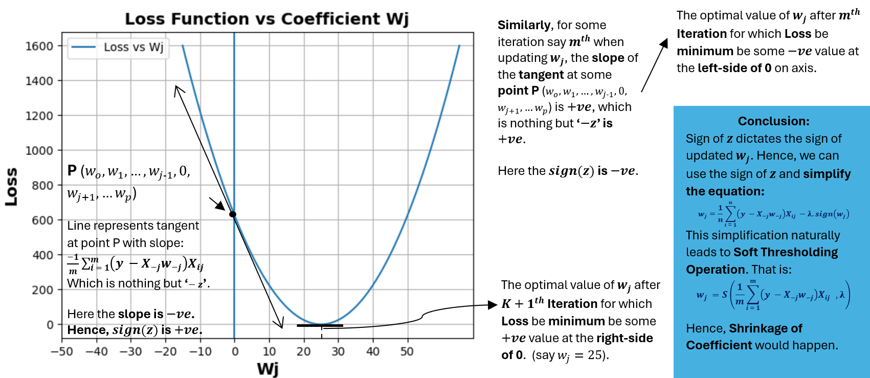
Let's say the slope of the tangent at point $P (w_0^k, w_1^k, \dots, w_{j - 1}^k, 0, w_{j + 1}^k, \dots, w_p^k)$ on the Loss curve in $p+2$ dimensional space is some negative slope.

$\hspace{3.5cm} \frac{\partial}{\partial w_j} \left( L(w) \right) \bigg|_{P = (w_0^k, w_1^k, \dots, w_{j - 1}^k, 0, w_{j + 1}^k, \dots, w_p^k, \text{Loss})} = \text{some negative value}$

That means, $-z$ is $-ve$ and hence $z$ is $+ve$. The optimal value of $w_j$ for which loss be minimum is some positive value at the right-side of $0$.

$\hspace{1.5cm} \frac{\partial}{\partial w_j} \left( L(w) \right) \bigg|_{P = (w_0^k, w_1^k, \dots, w_{j - 1}^k, 0, w_{j + 1}^k, \dots, w_p^k, \text{Loss})} = -z = \text{some negative value}$

$\hspace{4.5cm} z = \text{some positive value} \rarr \text{sign}(z) = +ve$

Check the below graph. Showing relationship between $w_j$ and Loss in 2-D plot:

Similarly, if the slope of the tangent at point $P (w_0^k, w_1^k, \dots, w_{j - 1}^k, 0, w_{j + 1}^k, \dots, w_p^k)$ on the Loss curve in $p+2$ dimensional space is some positive slope.

$\hspace{3.5cm} \frac{\partial}{\partial w_j} \left( L(w) \right) \bigg|_{P = (w_0^k, w_1^k, \dots, w_{j - 1}^k, 0, w_{j + 1}^k, \dots, w_p^k, \text{Loss})} = \text{some positive value}$

That means, $-z$ is $+ve$ and hence $z$ is $-ve$. The optimal value of $w_j$ for which loss be minimum is some negative value at the left-side of $0$.

$\hspace{1.5cm} \frac{\partial}{\partial w_j} \left( L(w) \right) \bigg|_{P = (w_0^k, w_1^k, \dots, w_{j - 1}^k, 0, w_{j + 1}^k, \dots, w_p^k, \text{Loss})} = -z = \text{some positive value}$

$\hspace{4.5cm} z = \text{some negative value} \rarr \text{sign}(z) = -ve$

NOTE: Irrespective of $\text{sign}(w_j)$ from kth optimization iteration, $\text{sign}(w_j)$ after $k + 1^{th}$ iteration can be determined by $\text{sign}{z}$.

You see, in both the cases $\text{sign}(z)$ aligns with the sign of updated $w_j$.

Conclusion: Sign of $z$ dictates the sign of updated $w_j$.

Hence, we can use the sign of $z$ and simplify the equation:

$\hspace{3.5cm} \boxed{w_j = \frac{1}{n} \sum_{i = 1}^{n} \left( y_i - X_{i-j} w_{-j} \right) X_{ij} - \lambda \operatorname{sign}(w_j)}$

This simplification naturally leads to Soft Thresholding Operation. That is:

$\hspace{3.5cm} \boxed{ \quad w_j = \text{Soft Thresholding} \left( \frac{1}{n} \sum_{i = 1}^{n} \left( y_i - \mathbf{X}_{i-j} \mathbf{w}_{i-j} \right) X_{ij}, \, \lambda \right) \quad}$

$\hspace{5.5cm} \boxed{ \quad w_j = \text{Soft Thresholding} \left( z, \, \lambda \right) \quad}$

Hence, shrinkage of coefficient would happen in Lasso Regression.

Thanks for reading! Do check out my other posts. Happy Learing.