In this last post of Regularization trilogy, we'll bind things up and explore the last regularization technique - Elastic-Net Regularization. How it works? Optimization technique used for solution finding? How it creates more flexible, robust and interpretable solution then vanilla Lasso and Ridge Regularization. Geometric interpretations of Elastic-Net Regularization. Let's jump in.

Before we see Elastic-Net Regularization. Let's take a quick look at the comparison between Lasso and Ridge Regularization. Would be a nice revision too.

Lasso Vs Ridge - Quick Recap

Below we are making comparison between Ridge and Lasso regression on some of their key aspects.

Aspect	Ridge Regression	Lasso Regression
Objective Function	$\min_{w} \left\{\vert{}y-Xw\vert{}_{2}^{2} + \lambda\vert{}w\vert{}_{L2}^{2}\right\}$	$\min_{w} \left\{\vert{}y-Xw\vert{}_{2}^{2} + \lambda\vert{}w\vert{}_{L1}\right\}$
Penalty Type	$L2$ norm (squared weights)	$L1$ norm (absolute weights)
Effect of Penalty	Shrinks all coefficients toward zero, but never zeroes them out entirely	Shrinks some coefficients exactly to zero — leading to Feature Selection
Sparsity	No Sparsity; all features are kept and just shrunked	creates sparse solutions — some weights become exactly zero
Feature Selection	No FS	Yes. Remove weak features.
Constraint's Geometry	Circular / spherical constraint shaped (smooth curve prevent exact zeros)	Diamond / rhombus shaped constraint (sharp corners enable exact zeros)
Optimization Landscape	Smooth, differentiable	Non-differentiable at zero (due to L1-penalty), handled via coordinate descent optimization
Behaviour with Correlated Predictors	Spreads weights among correlated predictors	Tends to pick one (with strongest signal) and zero out others
Bias-Variance Trade-off	Reduces variance at the cost of some bias	Also reduces variance, but often introduces more bias due to zeroing out coefficients
Preferred When	All features are relevant; no strong need for feature selection	Many features availble; some are irrelevant; when needed more interpretability or sparsity
Solution Form	Closed-form solution exists (with matrix inversion)	No closed-form solution; solved via iterative Coordinate Descent based optimization
Computation	Slightly more efficient (closed-form for small data)	Slower but scalable

Geometric Intuition of Lasso and Ridge

Ridge Regression: L2 constraint boundary is a circle (in 2D) or sphere (in nD). The point of minima is one where MSE contour rings touches the constraint boundary, and this point is likely be on the smooth curve of constraint boundary away from axes. Hence, coefficients reduce but no zero coefficients.

Lasso Regression: L1 constraint boundary is a diamond (in 2D) or cross-polytope/rhombus (in nD). The point of minima is one where MSE contour rings touches the constraint boundary, and this point is likely be on the sharp corners of constraint boundary on the axes. Hence, many coefficients are reduced to exact zero.

Note: As $\lambda$ increases, regularization strength increases and hence the shrinkage.

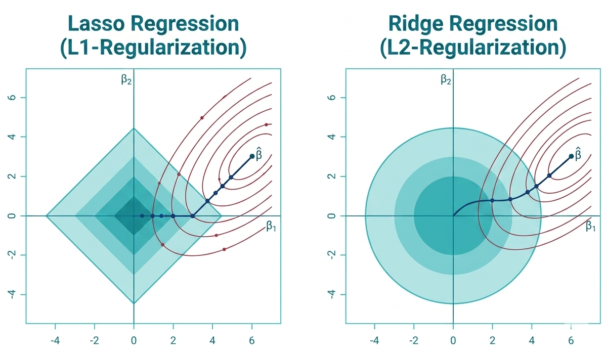
Geometric Intuition of i. Lasso (left) and ii. Ridge Regression (right)

Intuition Behind Shrinkage:

Ridge says: “All features are useful; let's just weaken their influence to prevent overfitting.”
Lasso says: Gotta' be selective! — keep the features that matter, and omit the rest.”

Let's conclude now. Solution where impact from all the input features is necessary, we use Ridge. On high-dimensional data like genetics data, use Lasso. If intepretability is top-most priority, then we need simpler solution, use Lasso. If data has correlated features then use Ridge - for keeping all the correlated features and grouping them togther, or use Lasso - to keep only the most impactful one.

What if I need the best of both? Let's see that.

Elastic-Net Regression

Elastic Net Regression is a regularized regression algorithm that linearly combines the penalties of Lasso (L1) and Ridge (L2) Regression. It is particularly useful when there are high-dimensional datasets or correlated features.

The Elastic-net estimates the regression coefficients by minimizing the following objective function:

$\hspace{1.5cm} \boxed{ \quad L(w) = \underbrace{\frac{1}{n}\sum_{i=1}^{n}(y_i-X_i.w)^2}_{\text{Prediction Error}} + \lambda. \left[ \underbrace{\alpha . \sum_{j=1}^{p}|w_j|}_{\text{L1 Penalty}} + \underbrace{\frac{1 - \alpha}{2} . \sum_{j=1}^{p}|w_j^2|}_{\text{L2 Penalty}} \right] \quad}$

where:

$\sum(y_i-X_i.w)^2$ → Mean Squared Error (MSE)
$\sum|w_j|$ → L1 Penalty (sum of absolute values)
$\sum|w_j^2|$ → L2 Penalty (sum of squares)
$\lambda \geq 0$ → Strength of regularization
$\alpha$ → $\in [0,1]$ ; balances Lasso and Ridge

NOTE:

α = 1: Lasso regression; α = 0: Ridge regression; And 0 < α < 1: Elastic-net regression
The intercept $w_0$ is not included in the Penalty Term.

Advantages of Elastic-net

Combines the benefits of Lasso and Ridge regularization.
Performs feature selection (like Lasso).
Handles multicollinearity well (like Ridge).
Encourages grouping effect for highly correlated features by binding them together.

Mathematical Solution

Loss Function can be given as:

$\hspace{1.5cm} L(w) = \frac{1}{2n}\sum_{i=1}^{n}(y_i-X_i.w)^2+ \lambda. \left[ \alpha . \sum_{j=1}^{p}|w_j| + \frac{1 - \alpha}{2} . \sum_{j=1}^{p}|w_j^2| \right]$

Coordinate Descent is the commonly used optimization algorithm to find the optimal solution for a Elastic-net Regression, especially when dealing with high-dimensional data.

Why Coordinate Descent? Loss function of Elastic-net involves a non-differentiable L1-norm term (due to absolute values), which makes gradient-based optimization harder. Coordinate Descent clears this hurdle by optimizing one coefficient at a time while holding others fixed.

How Coordinate Descent Works for Elastic-net

Its very similar to Lasso use case. At each optimization step only one coefficient is updated. For a coefficient $w_j \text{ where, } j = 1, 2, ..., p$ , at $k^{th}$ optimization step:

Hold all other coefficients fixed at values from $k-1^{th}$ optimization step.
Update $w_j$ using a soft-thresholding based update rule derived from partial derivatives and subgradients of the loss function.

$\hspace{2cm} \boxed{ \quad w_j(\text{new}) = \frac{\text{Soft Thresholding} \left( \frac{1}{n} \sum_{i = 1}^{n} \left( y_i - \mathbf{X}_{-j} \mathbf{w}_{-j} \right) X_{ij}, \, \lambda\alpha \right)}{\frac{1}{n} \sum_{i = 1}^{n} X_{ij}^2 + \lambda(1-\alpha)} \quad}$

$\quad$

Since, input features are normalized, $\frac{1}{n} \sum_{i = 1}^{n} X_{ij}^2 = 1$ . Simpler form be:

$\hspace{3cm} \boxed{ \quad w_j(\text{new}) = \frac{\text{Soft Thresholding} \left( z, \, \lambda\alpha \right)}{ 1 + \lambda(1-\alpha)} \quad}$

where:

Let $\frac{1}{n} \sum_{i = 1}^{n} \left( y_i - \mathbf{X}_{-j} \mathbf{w}_{-j} \right) X_{ij} \rarr$ be $z$ ; marginal correlation with residuals - measure of explainability of feature $X_j$ in regression
$\lambda$ and $\alpha \rarr$ Model hyperparameters

QUICK NOTE: - How Soft Thresholding Operator works:

$\hspace{2.2cm} \boxed{ \quad \text{Soft Thresholding}(z, \lambda\alpha) = \begin{cases} z - \lambda\alpha & \text{if } z > \lambda\alpha \\ z + \lambda\alpha & \text{if } z < -\lambda\alpha \\ 0 & \text{if } |z| \leq \lambda\alpha \end{cases} \quad}$

$\quad$

Most implementations (like scikit learn's -> sklearn.linear_model.ElasticNet) under the hood use Coordinate Descent based optimization for finding the optimal solution. Due to its efficiency and simplicity for problems with sparse or large feature spaces.

Geometric Intuition

For geometroc intuition, we must consider the solution finding for Elastic-net regression, a constrained optimization problem. This helps us visualize how Elastic-net balances between "sparsity" (Lasso) and "shrinkage" (Ridge).

Instead of minimizing a penalized loss function, we can reframe Elastic-net loss minimization as the following constrained optimization problem (COP):

$\hspace{2.2cm} \boxed{ \quad \underset{w}{\operatorname{min}} |y - Xw|_2^2 \quad \textbf{ subject to } \quad \left[ \alpha|w|_1 + (1 - \alpha)|w|^2_2 \right] \leq t \quad }$

where:

$|w|_1$ is the L1 norm (encourages sparsity),
$|w|^2_2$ is the L2 norm (encourages small, non-zero coefficients),
$\alpha \in [0,1]$ balances the two penalties,
$t$ controls the size of the constraint region (i.e., the “budget” for the coefficients); scales up and down the constraint region; smaller $t$ cooresponds to large $\lambda$ and vice verse.

Let's see how this span out geometrically.

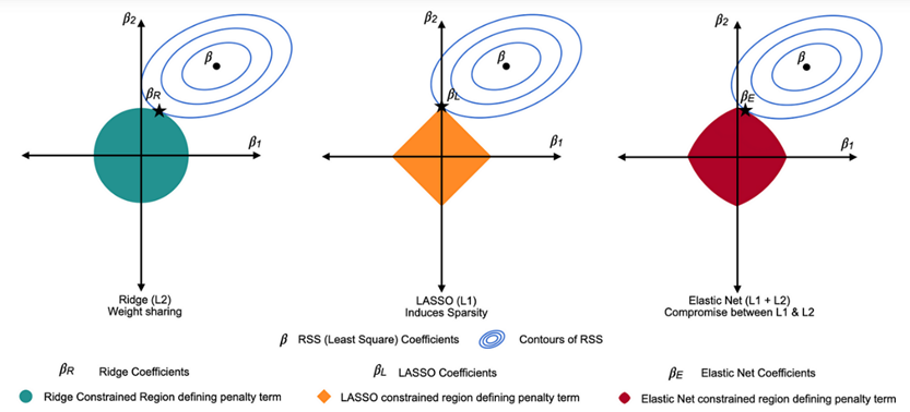
Geometric Intuition of i. Ridge (left), ii. Lasso (center) and iii. Elastic-net Regression (right)

The MSE part of the COP $(|y - Xw|_2^2)$ is a smooth, convex hyperbola. It can be shown as elliptical contour rings in 2D, centred around the OLS solution, the point where overfitting occurs.

The constraint region defined by the Elastic-net penalty is a combination of constraint boundaries of Lasso and Ridge regression.

Diamond (L1) → where sharp corners encourage zeros (like Lasso).
Circle (L2) → smooth shrinkage (like Ridge).

The constraint region defined by the Elastic-net penalty looks like a diamond being puffed out from the sides, into a rounder shape. The optimal solution is the point where the elliptical contours just touches the constraint region.

What Makes Elastic-net Special?

Corners in the constraint region encourage sparse solutions.
Smooth rounded sides weed-out instability when predictors are highly correlated, giving it the grouping effect (binding correlated variables together).

Hurray! We are done with all the three regularization techniques in great depth and how they apply in linear regression to optimize it. For any query and discussion, feel free to reach out via socials.

Thanks for reading!